42 accept labels in formulas excel 2013

Adding rich data labels to charts in Excel 2013 | Microsoft 365 Blog To add a data label in a shape, select the data point of interest, then right-click it to pull up the context menu. Click Add Data Label, then click Add Data Callout . The result is that your data label will appear in a graphical callout. In this case, the category Thr for the particular data label is automatically added to the callout too. Excel 2013: Label deconfliction in labeled scatter plot This formula then goes into G2 to create the series with labels below the point, which is all remaining values: =IF (ISERROR (F2),E2,NA ()) One trick is just required to make the autofilter work on the data.

IFS Function in Excel 2016, 2013, 2010 and 2007 - Office PowerUps Excel 365 or Excel 2019 introduced a new function called IFS. You can add an IFS function in Excel 2016, 2013 or your copy of Excel 2010, or 2007 with the Excel PowerUps add-in. This IFS function in Excel 2016 (or earlier) allows you to specify a series of conditions easily in a single function without having to nest several IF functions.

Accept labels in formulas excel 2013

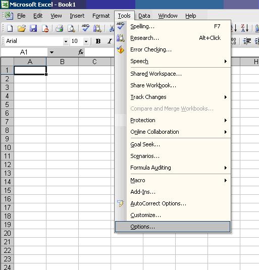
How to Use the AutoSum Feature in Microsoft Excel 2013 Excel will select a range of adjacent cells for you. If Excel choose the wrong range of cells, just use your mouse to click and drag over the correct range of cells to use in the formula. 2. Click the "AutoSum" button again or press the "Enter" key on your keyboard to accept the formula. 3. Names in formulas - support.microsoft.com Select the cell, range of cells, or nonadjacent selections that you want to name. Click the Name box at the left end of the formula bar. Name box Type the name you want to use to refer to your selection. Names can be up to 255 characters in length. Press ENTER. Note: You cannot name a cell while you are changing the contents of the cell. How to mail merge and print labels from Excel - Ablebits You are now ready to print mailing labels from your Excel spreadsheet. Simply click Print… on the pane (or Finish & Merge > Print documents on the Mailings tab). And then, indicate whether to print all of your mailing labels, the current record or specified ones. Step 8. Save labels for later use (optional)

Accept labels in formulas excel 2013. How to Assign a Name to a Range of Cells in Excel To assign a name to a range of cells, select the cells you want to name. The cells don't have to be contiguous. To select non-contiguous cells, use the "Ctrl" key when selecting them. Click the mouse in the "Name Box" above the cell grid. Type a name for the range of cells in the box and press "Enter". 4 steps: How to Create Waterfall Charts in Excel 2013 - Data Cycle ... Add data labels by right-clicking one of the series and selecting "Add data labels…" Add labels to each of the series apart from the invisible column. Select the data labels and make them bold, change colour as appropriate. The finished chart should look something similar to the one below. Download the completed version here. grab user attention Use Excel Slicer Selection in Formulas - My Online Training Hub In the dialog box (image below), select the field you want to insert a Slicer for: Note: if you already have a Slicer inserted, you can connect it to the quasi PivotTable by right-clicking the Slicer > Connections > check the box for the quasi PivotTable. I'll also change my Slicer caption to say "Select One" to give some guidance to the user. excel - For each loop with labels and variables - Stack Overflow Then you can loop through the labels, but do a check on the values. For i=lbound (labelarray) to ubound (labelarray) If valarray (i) > 0 Then Managementsitzung.Controls (labelarray (i) & i1).Caption = valarray (i) Else Managementsitzung.Controls (labelarray (i) & i1).Caption = "-" End If Next i Share answered Aug 22, 2016 at 14:36 Matt Cremeens

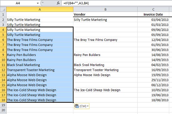
Jan's Excel Format & Arrange (97- 2003): Exercises [Hint: Cut and Insert Cells.] There should be a blank row between the Totals and Expenses rows. Move the column labels from below Expenses to above Income. Insert: Between the columns Category and Budget, insert 2 columns. Label the columns Budget Quantity and Budget Cost each and wrap the text. How to add data labels from different column in an Excel chart? In the Format Data Labels pane, under Label Options tab, check the Value From Cells option, select the specified column in the popping out dialog, and click the OK button. Now the cell values are added before original data labels in bulk. 4. Go ahead to untick the Y Value option (under the Label Options tab) in the Format Data Labels pane. How to use AutoFill in Excel - all fill handle options - Ablebits In Excel 2010-2013 click File -> Options -> Advanced -> scroll to the General section to find the Edit Custom Lists… button. Since you already selected the range with your list, you will see its address in the Import list from cells: field. Press the Import button to see your series in the Custom Lists window. What Are the Rules for Excel Names? - Contextures Blog There are rules for Excel Names, and here's what Microsoft says is allowed. It seems clear, but a few of the rules aren't as ironclad as they look: The first character of a name must be one of the following characters: letter. underscore (_) backslash (\). Remaining characters in the name can be. letters. numbers.

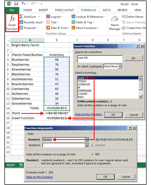
Excel 2016 - How to Use Formulas and Functions To do this, we are going to click Insert Function on the Ribbon under the Formulas tab. Once again, we enter "average of cells" in the "Search for a Function field," then click the Go button. Select Average, then click OK. Excel prompts us for our arguments. The arguments are the cells or values that we want to use to calculate the function. How to Use Templates and Outlines in Excel 2013 Click the Add button. Enter a name for the view in the Name box. Now go to Include In View and select the settings that you want to include. Click OK. To apply a custom view, click the View tab again, then click Custom Views. Select the name of your view in the Custom Views dialogue box. Click the Show button. Named Ranges in Excel: See All Defined Names (Incl. Hidden Names) The built-in Name Manager in Excel doesn't show all defined names. Why not showing all names is a problem. Solution 1: Access named ranges manually. Solution 2: Use a VBA macro to see all named ranges. VBA macros to make all names visible. VBA macro to remove all names. VBA macro to remove all hidden names. Understanding Date-Based Axis Versus Category-Based Axis in Trend ... Press Ctrl+; to enter today's date in the cell. Again, select cell B5. Press Ctrl+1 to display the Format Cells dialog. Change the number format from a date to a number. Your date changes to a number in the 40,000 to 42,000 range, assuming you are reading this in the 2013-2015 time period. This might sound like a hassle, but it is worth it.

How to Use Excel Like a Pro: 18 Easy Excel Tips, Tricks, & Shortcuts

Excel Workbook wouldn't accept cumulated total formula (Eg. - Microsoft ... Excel Workbook wouldn't accept cumulated total formula (Eg. =SUM ('Musoma Municipal:Butiama District'!D15) from its sheets. Hi, I have been using Excel over 20 years now though I can't say that I know Excel that much. I have recently denied by Excel to make formula that I have been using over four years now, work.

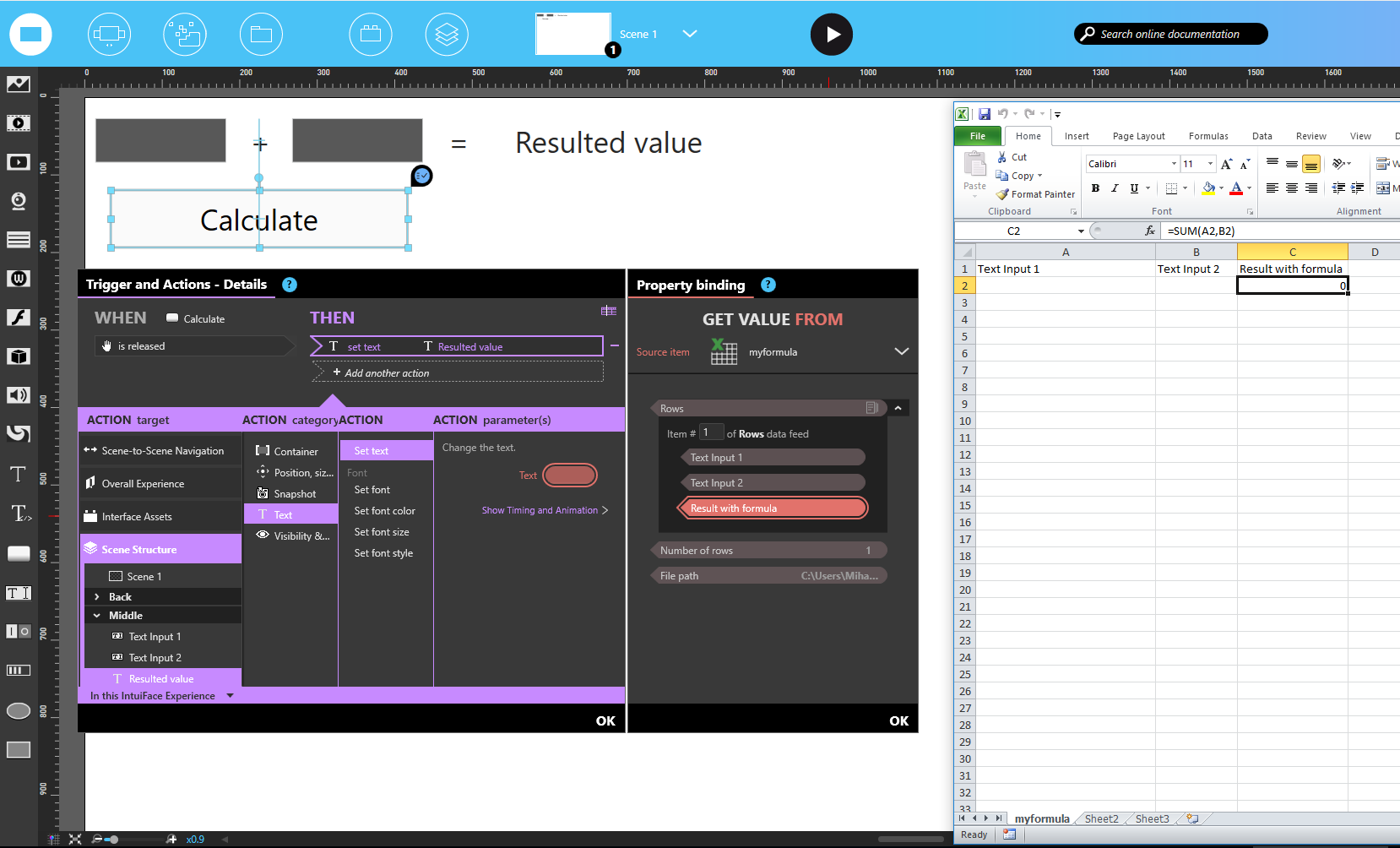
How to use Excel Formulas – Intuiface

Use defined names to automatically update a chart range - Office Microsoft Excel 97 through Excel 2003. On the Insert menu, click Chart to start the Chart Wizard. Click a chart type, and then click Next. Click the Series tab. In the Series list, click Sales. In the Category (X) axis labels box, replace the cell reference with the defined name Date. For example, the formula might be similar to the following ...

What formula do I use in Excel to get 04/15/2018 be this: 20180415? - Quora

Keep Your Formulas From Shifting In Excel - Business Insider Aug 2, 2013, 12:08 PM One of the best features in Excel is the ability to plug in a formula and then easily drag it into new cells and have it automatically shift to the corresponding cell values....

Using Labels to Simplify Your Excel 2003 Formulas

How to Convert a Formula to a Static Value in Excel 2013 To do this, click in the cell with the formula and select the part of the formula you want to convert to a static value and press F9. NOTE: When selecting part of a formula, be sure that you include the entire operand in your selection. The part of the formula you are converting must be able to be calculated to a static value.

How To Use Labels As References In MS Excel XP. - PCauthorities.com :PCauthorities.com

How to Print Labels From Excel - EDUCBA Navigate towards the folder where the excel file is stored in the Select Data Source pop-up window. Select the file in which the labels are stored and click Open. A new pop up box named Confirm Data Source will appear. Click on OK to let the system know that you want to use the data source. Again a pop-up window named Select Table will appear.

Excel Formula Help - IF Formulas

Excel- Labels, Values, and Formulas - WebJunction Simple Formula: Click the cell in which you want the answer (result of the formula) to appear. Press Enter once you have typed the formula. All formulas start with an = sign. Refer to the cell address instead of the value in the cell e.g. =A2+C2 instead of 45+57. That way, if a value changes in a cell, the answer to the formula changes with it.

Excel Formulas: Defining and Creating a Formula

Define and use names in formulas - support.microsoft.com Select Formulas > Create from Selection. In the Create Names from Selection dialog box, designate the location that contains the labels by selecting the Top row, Left column, Bottom row, or Right column check box. Select OK. Excel names the cells based on the labels in the range you designated. Use names in formulas

Insert Formula In Excel7 - Whatvwant

Enable or Disable Excel Data Labels at the click of a button - How To Select and to go Insert tab > Charts group > Click column charts button > click 2D column chart. This will insert a new chart in the worksheet. Step 2: Having chart selected go to design tab > click add chart element button > hover over data labels > click outside end or whatever you feel fit. This will enable the data labels for the chart.

Most Frequently used Basic Excel Formulas with Examples

How to Prevent or Disable Auto Fill in Table Formulas - Excel Campus The button appears to the right of the cell after you enter a formula in the Table column. There are three options on this menu. 1. Undo Calculated Column Undo Calculated Column accomplishes the same thing we've seen above with Ctrl + Z or Undo. 2. Stop Automatically Creating Calculated Columns

Your Excel formulas cheat sheet: 15 tips for calculations and common tasks – Sibanye-Stillwater

Excel 2013, Filter not working for all table content Select the "Table tools" ribbon that is displayed above the other ribbons. Select "Resize table" (at far left of Table tools ribbon). The resize dialog will be displayed. It will be obvious it only rows down to 468 are included in the table by the range shown by default as the current range of the table.

How are IF formulas used in Excel? - Quora

How to mail merge and print labels from Excel - Ablebits You are now ready to print mailing labels from your Excel spreadsheet. Simply click Print… on the pane (or Finish & Merge > Print documents on the Mailings tab). And then, indicate whether to print all of your mailing labels, the current record or specified ones. Step 8. Save labels for later use (optional)

Report Designer User Guide

Names in formulas - support.microsoft.com Select the cell, range of cells, or nonadjacent selections that you want to name. Click the Name box at the left end of the formula bar. Name box Type the name you want to use to refer to your selection. Names can be up to 255 characters in length. Press ENTER. Note: You cannot name a cell while you are changing the contents of the cell.

Share :