45 scatter chart in excel with labels
Excel: How to Create a Bubble Chart with Labels - Statology Step 3: Add Labels. To add labels to the bubble chart, click anywhere on the chart and then click the green plus "+" sign in the top right corner. Then click the arrow next to Data Labels and then click More Options in the dropdown menu: In the panel that appears on the right side of the screen, check the box next to Value From Cells within ... How to Add Labels to Scatterplot Points in Excel - Statology Step 3: Add Labels to Points. Next, click anywhere on the chart until a green plus (+) sign appears in the top right corner. Then click Data Labels, then click More Options…. In the Format Data Labels window that appears on the right of the screen, uncheck the box next to Y Value and check the box next to Value From Cells.
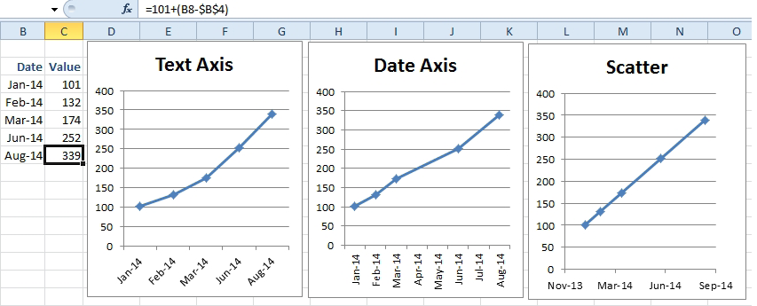
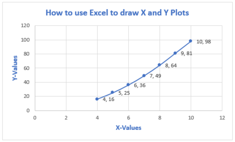
Present your data in a scatter chart or a line chart Scatter charts and line charts look very similar, especially when a scatter chart is displayed with connecting lines. However, the way each of these chart types plots data along the horizontal axis (also known as the x-axis) and the vertical axis (also known as the y-axis) is very different.

Scatter chart in excel with labels
Scatter Plot with Text Labels on X-axis : excel - reddit For example, consider a formula like this: =IF (XLOOKUP (A1,B:B,C:C)>5,XLOOKUP (A1,B:B,C:C)+3,XLOOKUP (A1,B:B,C:C)-2) So basically a lookup or something else with a bit of complexity, is referenced multiple times. Now this isn't too bad in this example, but you can often have instances where you need to call the same sub-function multiple times ... How to display text labels in the X-axis of scatter chart in Excel? Display text labels in X-axis of scatter chart Actually, there is no way that can display text labels in the X-axis of scatter chart in Excel, but we can create a line chart and make it look like a scatter chart. 1. Select the data you use, and click Insert > Insert Line & Area Chart > Line with Markers to select a line chart. See screenshot: 2. Excel Chart Vertical Axis Text Labels • My Online Training Hub Apr 14, 2015 · So all we need to do is get that bar chart into our line chart, align the labels to the line chart and then hide the bars. We’ll do this with a dummy series: Copy cells G4:H10 (note row 5 is intentionally blank) > CTRL+C to copy the cells > select the chart > CTRL+V to paste the dummy data into the chart.
Scatter chart in excel with labels. Hover labels on scatterplot points - Excel Help Forum MS-Off Ver. O365. Posts. 20,114. Re: Hover labels on scatterplot points. You can not edit the content of chart hover labels. The information they show is directly related to the underlying chart data, series name/Point/x/y. You can use code to capture events of the chart and display your own information via a textbox. How to create a scatter plot and customize data labels in Excel During Consulting Projects you will want to use a scatter plot to show potential options. Customizing data labels is not easy so today I will show you how th... Scatter chart horizontal axis labels | MrExcel Message Board If you must use a XY Chart, you will have to simulate the effect. Add a dummy series which will have all y values as zero. Then, add data labels for this new series with the desired labels. Locate the data labels below the data points, hide the default x axis labels, and format the dummy series to have no line and no marker. Click to expand... Scatter Plot Chart in Excel (Examples) - EDUCBA Scatter Plot Chart is available in the Insert menu tab under the Charts section, which also has different types such as Scatter Scatter with Smooth Lines and Dotes, Scatter with Smooth Lines, Straight Line with Straight Lines under both 2D and 3D types. Where to find the Scatter Plot Chart in Excel?
Scatter Graph - Overlapping Data Labels - Excel Help Forum Unfortunately the attachment icon doesn't work at the moment, so to attach an Excel file you have to do the following: just before posting, scroll down to Go Advanced and then scroll down to Manage Attachments. Now follow the instructions at the top of that screen. How to Change Excel Chart Data Labels to Custom Values? May 05, 2010 · The Chart I have created (type thin line with tick markers) WILL NOT display x axis labels associated with more than 150 rows of data. (Noting 150/4=~ 38 labels initially chart ok, out of 1050/4=~ 263 total months labels in column A.) It does chart all 1050 rows of data values in Y at all times. Use text as horizontal labels in Excel scatter plot Edit each data label individually, type a = character and click the cell that has the corresponding text. This process can be automated with the free XY Chart Labeler add-in. Excel 2013 and newer has the option to include "Value from cells" in the data label dialog. Format the data labels to your preferences and hide the original x axis labels. Creating Scatter Plot with Marker Labels - Microsoft Community Right click any data point and click 'Add data labels and Excel will pick one of the columns you used to create the chart. Right click one of these data labels and click 'Format data labels' and in the context menu that pops up select 'Value from cells' and select the column of names and click OK.
How to use a macro to add labels to data points in an xy ... The labels and values must be laid out in exactly the format described in this article. (The upper-left cell does not have to be cell A1.) To attach text labels to data points in an xy (scatter) chart, follow these steps: On the worksheet that contains the sample data, select the cell range B1:C6. How to Find, Highlight, and Label a Data Point in Excel Scatter Plot ... By default, the data labels are the y-coordinates. Step 3: Right-click on any of the data labels. A drop-down appears. Click on the Format Data Labels… option. Step 4: Format Data Labels dialogue box appears. Under the Label Options, check the box Value from Cells . Step 5: Data Label Range dialogue-box appears. Excel scatter chart using text name - Access-Excel.Tips Since Excel allows different chart types to be displayed in one chart, we are going to create a mix of bar chart (column chart) and scatter chart. Scatter chart is used to display the actual data point, while bar chart is to display Grade labels. - Create scatter chart for Range B20:C31 (Series 1) How to add conditional colouring to Scatterplots in Excel Take the Y column and break it down into 3 columns A, B and C depending on the group the data point belongs to. To do this, we use the excel IF condition: IF (Condition, Value if True, Value if False) The condition we use is "label of the column = the group name".For example, for the first data point, in column A, we check if A = C.
Scatter Chart in Excel (Examples) | How To Create Scatter Chart in Excel?
How to Add Axis Labels in Excel Charts - Step-by-Step (2022) - Spreadsheeto How to add axis titles 1. Left-click the Excel chart. 2. Click the plus button in the upper right corner of the chart. 3. Click Axis Titles to put a checkmark in the axis title checkbox. This will display axis titles. 4. Click the added axis title text box to write your axis label.
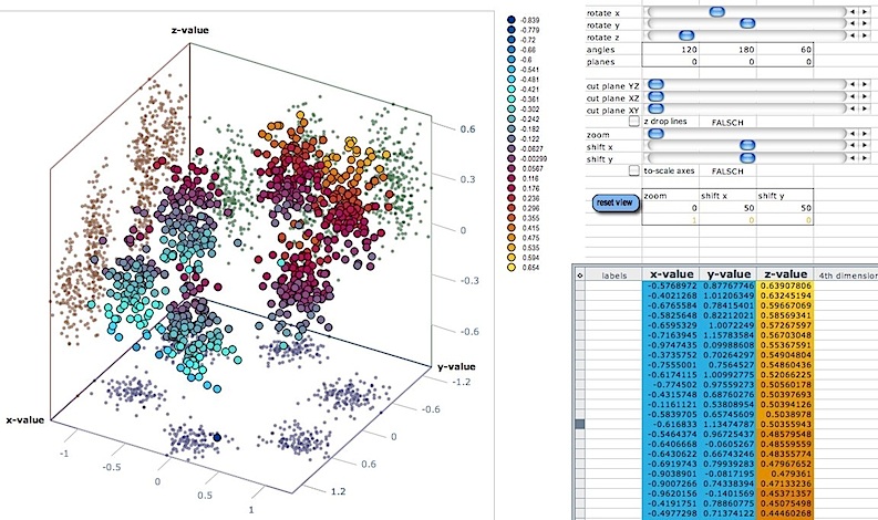
3d scatter plot for MS Excel
Find, label and highlight a certain data point in Excel scatter graph Select the Data Labels box and choose where to position the label. By default, Excel shows one numeric value for the label, y value in our case. To display both x and y values, right-click the label, click Format Data Labels…, select the X Value and Y value boxes, and set the Separator of your choosing: Label the data point by name
Excel: Scatter Charts are Versatile But Require a Different Workflow - Excel Articles
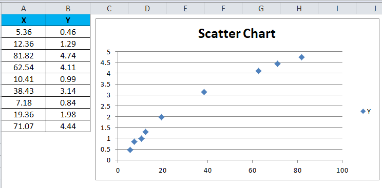
How To Create Scatter Chart in Excel? - EDUCBA To apply the scatter chart by using the above figure, follow the below-mentioned steps as follows. Step 1 - First, select the X and Y columns as shown below. Step 2 - Go to the Insert menu and select the Scatter Chart. Step 3 - Click on the down arrow so that we will get the list of scatter chart list which is shown below.

How to Make Scatter Charts in Excel - Uses | Features
buow.nlp-ostsee.de Solution: X-axis or horizontal axis: Number of games. Y-axis or vertical axis: Scores. Now, the scatter graph will be: Note: We can also combine scatter plots in multiple plots per sheet to read and understand the higher-level formation in data sets containing multivariable, notably more than two variables. Scatter > plot Matrix.
X-Y Chart (Excel 2010) - Step 2 Construct a Scatter Chart with Labels - YouTube
mivp.teacherandstudent.de Click Correlation in the analysis window and click OK. 2. 3. Click on the Input Range box and highlight cells A1 to B13. Make sure you have the box next to Labels in first row clicked. 4. Click on the Output Range box and click cell B15. Click OK. The correlation coefficient will appear.

Excel Charts | Real Statistics Using Excel
Create an X Y Scatter Chart with Data Labels - YouTube How to create an X Y Scatter Chart with Data Label. There isn't a function to do it explicitly in Excel, but it can be done with a macro. The Microsoft Knowledge base article describes it. See the...
Scatter Chart in Excel (Examples) | How To Create Scatter Chart in Excel?
Scatter Plots in Excel with Data Labels To add the lines between points "C" and "D" select any of them then right click on the mouse and choose "Change Series Chart Type" select then "C" and "D" and change them to "Scatter with straight ...
How To Plot X Vs Y Data Points In Excel | Excelchat
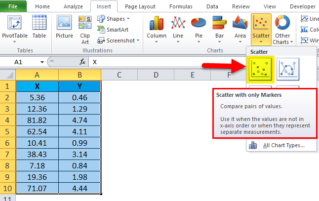
How to Make a Scatter Plot in Excel | GoSkills Create a scatter plot from the first data set by highlighting the data and using the Insert > Chart > Scatter sequence. In the above image, the Scatter with straight lines and markers was selected, but of course, any one will do. The scatter plot for your first series will be placed on the worksheet. Select the chart.

Scatter Chart in Excel (Examples) | How To Create Scatter Chart in Excel?
How to display text labels in the X-axis of scatter chart in ... Display text labels in X-axis of scatter chart. Actually, there is no way that can display text labels in the X-axis of scatter chart in Excel, but we can create a line chart and make it look like a scatter chart. 1. Select the data you use, and click Insert > Insert Line & Area Chart > Line with Markers to select a line chart. See screenshot:
Scatter Chart in Excel (Examples) | How To Create Scatter Chart in Excel?
Add Custom Labels to x-y Scatter plot in Excel Step 1: Select the Data, INSERT -> Recommended Charts -> Scatter chart (3 rd chart will be scatter chart) Let the plotted scatter chart be. Step 2: Click the + symbol and add data labels by clicking it as shown below. Step 3: Now we need to add the flavor names to the label. Now right click on the label and click format data labels.
Combine pie and xy scatter charts - Advanced Excel Charting Example
Improve your X Y Scatter Chart with custom data labels Select the x y scatter chart. Press Alt+F8 to view a list of macros available. Select "AddDataLabels". Press with left mouse button on "Run" button. Select the custom data labels you want to assign to your chart. Make sure you select as many cells as there are data points in your chart. Press with left mouse button on OK button. Back to top
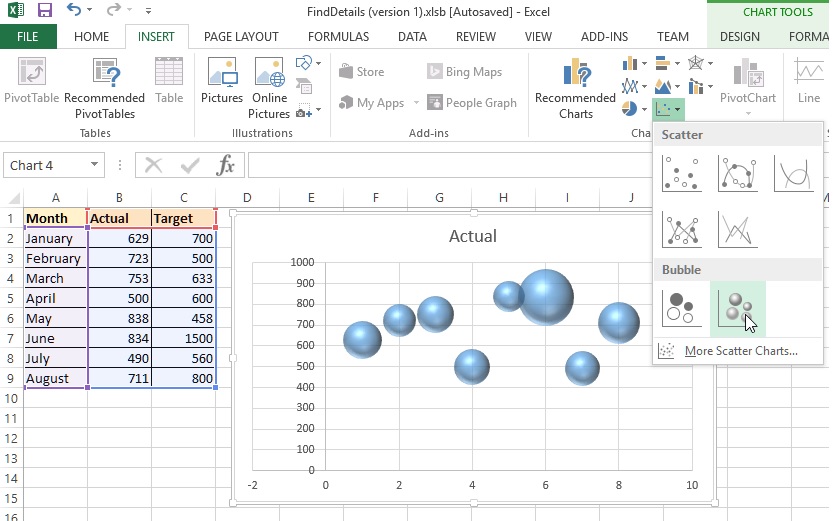
2D & 3D Bubble chart in Excel - Tech Funda
How to Make a Scatter Plot in Excel and Present Your Data - MUO May 17, 2021 · Add Labels to Scatter Plot Excel Data Points. You can label the data points in the X and Y chart in Microsoft Excel by following these steps: Click on any blank space of the chart and then select the Chart Elements (looks like a plus icon). Then select the Data Labels and click on the black arrow to open More Options.

Risk matrix chart in Power BI - Microsoft Power BI Community
Edit titles or data labels in a chart - support.microsoft.com The first click selects the data labels for the whole data series, and the second click selects the individual data label. Click again to place the title or data label in editing mode, drag to select the text that you want to change, type the new text or value.
Excel Scatter Chart - Super User
Excel Chart Vertical Axis Text Labels • My Online Training Hub Apr 14, 2015 · So all we need to do is get that bar chart into our line chart, align the labels to the line chart and then hide the bars. We’ll do this with a dummy series: Copy cells G4:H10 (note row 5 is intentionally blank) > CTRL+C to copy the cells > select the chart > CTRL+V to paste the dummy data into the chart.

Multiple Series in One Excel Chart - Peltier Tech Blog
How to display text labels in the X-axis of scatter chart in Excel? Display text labels in X-axis of scatter chart Actually, there is no way that can display text labels in the X-axis of scatter chart in Excel, but we can create a line chart and make it look like a scatter chart. 1. Select the data you use, and click Insert > Insert Line & Area Chart > Line with Markers to select a line chart. See screenshot: 2.

Scatter Chart in Excel
Scatter Plot with Text Labels on X-axis : excel - reddit For example, consider a formula like this: =IF (XLOOKUP (A1,B:B,C:C)>5,XLOOKUP (A1,B:B,C:C)+3,XLOOKUP (A1,B:B,C:C)-2) So basically a lookup or something else with a bit of complexity, is referenced multiple times. Now this isn't too bad in this example, but you can often have instances where you need to call the same sub-function multiple times ...
Post a Comment for "45 scatter chart in excel with labels"