41 add data labels to pivot chart

how to add data labels into Excel graphs 10 Feb 2021 — Right-click on a point and choose Add Data Label. You can choose any point to add a label—I'm strategically choosing the endpoint because that's ... Automatic Row And Column Pivot Table Labels - How To Excel At Excel Select the data set you want to use for your table The first thing to do is put your cursor somewhere in your data list Select the Insert Tab Hit Pivot Table icon Next select Pivot Table option Select a table or range option Select to put your Table on a New Worksheet or on the current one, for this tutorial select the first option Click Ok

How to Add a Column to a Pivot Table - Excel Tutorials - OfficeTuts Excel Add a Column to a Pivot Table. Now that we have our data into the Pivot Table, we will put players into the row field and averages of points into the value fields: If you, for whatever reason, wanted a different value (for example, a total sum of points) all you have to do is click the field in values (in this case Average of Points) and select ...

Add data labels to pivot chart

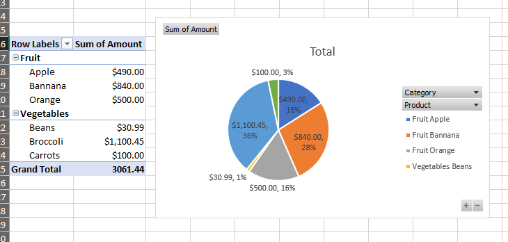
Add Value Label to Pivot Chart Displayed as Percentage If you use the hidden line method: How to Add Total Data Labels to the Excel Stacked Bar Chart and then use the code mentioned in post #2 to create boxes offset from the hidden line points, you should be able to place the additional labels where you want. You must log in or register to reply here. Similar threads E How to Make a Pie Chart in Excel & Add Rich Data Labels to The Chart! 7) With the data point still selected, go to Chart Tools>Format>Shape Styles and click on the drop-down arrow next to Shape Effects and select Shadow and choose Inner Shadow>Inside Diagonal Top Left. 8) With the one data point still selected, right-click this data point, and select Add Data Label>Add Data Callout as shown below. Display data point labels outside a pie chart in a paginated report ... To display data point labels inside a pie chart. Add a pie chart to your report. For more information, see Add a Chart to a Report (Report Builder and SSRS). On the design surface, right-click on the chart and select Show Data Labels. To display data point labels outside a pie chart. Create a pie chart and display the data labels. Open the ...

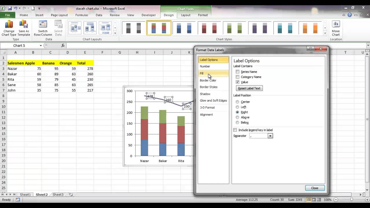
Add data labels to pivot chart. Create Dynamic Chart Data Labels with Slicers - Excel Campus You basically need to select a label series, then press the Value from Cells button in the Format Data Labels menu. Then select the range that contains the metrics for that series. Click to Enlarge Repeat this step for each series in the chart. If you are using Excel 2010 or earlier the chart will look like the following when you open the file. How to Add Total Data Labels to the Excel Stacked Bar Chart Step 4: Right click your new line chart and select "Add Data Labels" Step 5: Right click your new data labels and format them so that their label position is "Above"; also make the labels bold and increase the font size. Step 6: Right click the line, select "Format Data Series"; in the Line Color menu, select "No line" Step 7 ... Include Grand Totals in Pivot Charts • My Online Training Hub Step 5: Format the Chart. The Grand Total value is the top segment of the stacked column chart. We need to hide this, but first let's select the grand total series and add Data Labels > Inside Base: Next, with the grand total series still selected go to the Format tab > Shape Fill > No Fill. Hide the gridlines and vertical axis, and place the ... Adding rich data labels to charts in Excel 2013 | Microsoft 365 Blog First, I select my data label and I type some additional text to give context to the new number I'm about to add to the data label. Then, I right-click the data label to pull up the context menu. Note the Insert Data Label Field menu item. When I click Insert Data Label Field, Excel 2013 opens a dialog that gives me a few options to choose from.

How to Use Label Filters for Text in the Pivot Table? Step 1: The first step is to create a pivot table for the data. To know how to create a Pivot table please Click Here. Step 2: To add a field, Tick the checkbox before the field name in the PivotTable Fields panel. When you select the field name, the selected field name will be inserted into the pivot table. Pro Tip. Row Labels are used to ... Pivot Charts with Data Labels other than Values Click on data labels and use the right "arrow" to select that you want the information to appear above the bar. Then right click on the data label and select Format Data Labels, Under label options you have choices like Series name, Category name, etc. One spreadsheet to rule them all. One spreadsheet to find them. How to add data labels from different column in an Excel chart? Right click the data series in the chart, and select Add Data Labels > Add Data Labels from the context menu to add data labels. 2. Click any data label to select all data labels, and then click the specified data label to select it only in the chart. 3. How to add Data label in Stacked column chart of Pivot charts I'm tring to make a Pivot chart with stacked column graph. In where, i couldn't add data label for cumulative sum of value in Data label. Where i could only add data label to individual stacks in column graph. It found possible with normal stacked column chart without pivot chart.

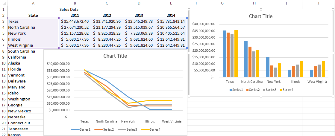
Excel charts: add title, customize chart axis, legend and data labels Click anywhere within your Excel chart, then click the Chart Elements button and check the Axis Titles box. If you want to display the title only for one axis, either horizontal or vertical, click the arrow next to Axis Titles and clear one of the boxes: Click the axis title box on the chart, and type the text. How to change/edit Pivot Chart's data source/axis ... - ExtendOffice Step 1: Select the Pivot Chart you will change its data source, and cut it with pressing the Ctrl + X keys simultaneously. Step 2: Create a new workbook with pressing the Ctrl + N keys at the same time, and then paste the cut Pivot Chart into this new workbook with pressing Ctrl + V keys at the same time. Step 3: Now cut the Pivot Chart from ... How to Add Rows to a Pivot Table: 9 Steps (with Pictures) - wikiHow Click anywhere in your pivot table. This opens the pivot table editor on the right side of Google Sheets. 3. Click Add under "Rows." It's in the left side of the pivot table editor. A list of fields will expand on the menu. 4. Click the name of the field you want to add as a row. Formal ALL data labels in a pivot chart at once Hi AaronSchmid ，. I go through the post, as per the article: Change the format of data labels in a chart, you may select only one data labels to format it. However, you may change the location of the data labels all at once, as you can see in screenshot below: I would suggest you vote for or leave your comments in the thread: Format Data ...

Creating Databound ADF Data Visualization Components

Add or remove data labels in a chart - support.microsoft.com In the upper right corner, next to the chart, click Add Chart Element > Data Labels. To change the location, click the arrow, and choose an option. If you want to show your data label inside a text bubble shape, click Data Callout. To make data labels easier to read, you can move them inside the data points or even outside of the chart.

How-to Use Data Labels from a Range in an Excel Chart - Excel Dashboard Templates

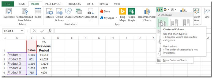
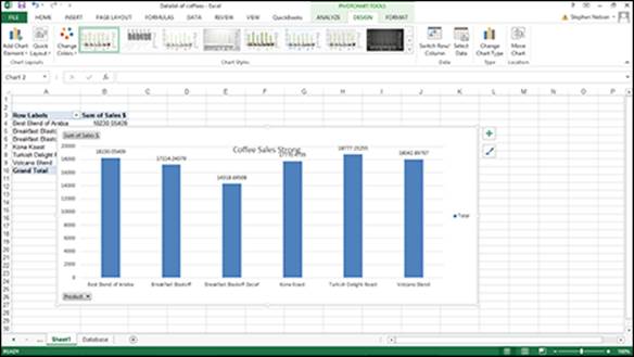
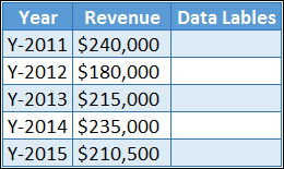
Data Labels in Excel Pivot Chart (Detailed Analysis) Adding Data Labels in Pivot Chart — To do this, go to Insert tab > Tables group. · Then in the dialog box, select the range of cells of the primary ...

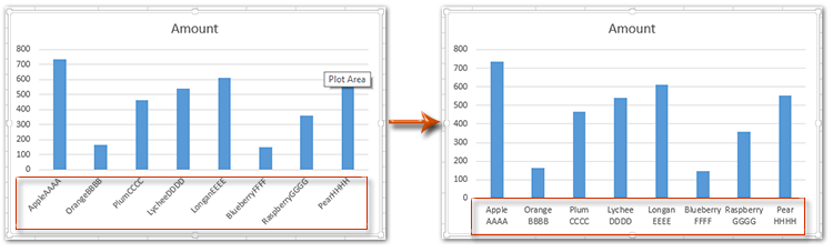
How to wrap X axis labels in a chart in Excel?

How to Add Data to a Pivot Table: 11 Steps (with Pictures) - wikiHow Open your pivot table Excel document. Double-click the Excel document that contains your pivot table. It will open. 2 Go to the spreadsheet page that contains your data. Click the tab that contains your data (e.g., Sheet 2) at the bottom of the Excel window. 3 Add or change your data.

Pivot Chart Data Label Help Needed - Microsoft Community

Adding Data Labels to a Chart Using VBA Loops - Wise Owl One way to do this is by manually adding data labels to the chart within Excel, but we're going to achieve the same result in a single line of code. To do this, add the following line to your code: 'make sure data labels are turned on FilmDataSeries.HasDataLabels = True

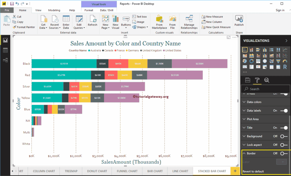
Format Stacked Bar Chart in Power BI

Add a DATA LABEL to ONE POINT on a chart in Excel Steps shown in the video above: Click on the chart line to add the data point to. All the data points will be highlighted. Click again on the single point that you want to add a data label to. Right-click and select ' Add data label ' This is the key step! Right-click again on the data point itself (not the label) and select ' Format data label '.

MS Excel 2013: Display the fields in the Values Section in multiple columns in a pivot table

Add a data label on Pivot Chart - social.technet.microsoft.com I have created a Pivot Chart for a data set & in the Vertical Bar I have a combined dataset which illustrates values of each parameter. When I add data labels it shows data labels for each parameter on the vertical bar but instead I would like to see a data label with the TOTAL for that ... · Hi, Please copy the TOTAL value into a new worksheet. For ...

Add label to Excel chart line • AuditExcel.co.za

How to Add Data Labels in Excel - Excelchat | Excelchat After inserting a chart in Excel 2010 and earlier versions we need to do the followings to add data labels to the chart; Click inside the chart area to display the Chart Tools. Figure 2. Chart Tools. Click on Layout tab of the Chart Tools. In Labels group, click on Data Labels and select the position to add labels to the chart.

image

How to Customize Your Excel Pivot Chart Data Labels - dummies To add data labels, just select the command that corresponds to the location you want. To remove the labels, select the None command. If you want to specify what Excel should use for the data label, choose the More Data Labels Options command from the Data Labels menu. Excel displays the Format Data Labels pane.

Add Total Label On Stacked Bar Chart In Excel - YouTube

Add a data label on Pivot Chart - social.technet.microsoft.com With ActiveChart With .SeriesCollection (1).Points (i) .HasDataLabel = True .DataLabel.Text = Worksheets ("Sheet2").Range ("a" & position_total).Value position_total = position_total + 1 End With End With Next End Sub Select the Pivot chart, then run the macro "data_label". Jaynet Zhang TechNet Community Support Monday, April 30, 2012 4:50 AM

How to Add Total Data Labels to the Excel Stacked Bar Chart – MBA Excel

Adding Data Labels to a Pivot Chart with VBA Macro I have a Pivot Table called PivotTable1 I have a chart called Cluster Review The range is dynamic can be different by import I want to add data labels to each series automatically (bearing in mind the number of series can change I have seen this code that someone else used and have inserted my...

Working with Multiple Data Series in Excel | Pryor Learning Solutions

Change the format of data labels in a chart To get there, after adding your data labels, select the data label to format, and then click Chart Elements > Data Labels > More Options. To go to the appropriate area, click one of the four icons ( Fill & Line, Effects, Size & Properties ( Layout & Properties in Outlook or Word), or Label Options) shown here.

How to group (two-level) axis labels in a chart in Excel?

Display data point labels outside a pie chart in a paginated report ... To display data point labels inside a pie chart. Add a pie chart to your report. For more information, see Add a Chart to a Report (Report Builder and SSRS). On the design surface, right-click on the chart and select Show Data Labels. To display data point labels outside a pie chart. Create a pie chart and display the data labels. Open the ...

How to Create Progress Charts (Bar and Circle) in Excel - Automate Excel

How to Make a Pie Chart in Excel & Add Rich Data Labels to The Chart! 7) With the data point still selected, go to Chart Tools>Format>Shape Styles and click on the drop-down arrow next to Shape Effects and select Shadow and choose Inner Shadow>Inside Diagonal Top Left. 8) With the one data point still selected, right-click this data point, and select Add Data Label>Add Data Callout as shown below.